scID
R library that enables identification of equivalent cell populations across single-cell RNA-seq datasets
This project is maintained by BatadaLab
Tutorial: Identification of equivalent cells across single-cell RNA-seq datasets
This tutorial is an example of using scID for mapping across two 10X datasets of E18 mouse brain single-cells and single-nuclei from cortex, hippocampus and subverticular zone. To speed-up preprocessing you can download the TPM-normalized data we have pre-computed.
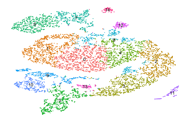
The reference cells can be grouped into 15 clusters as shown in the next plot.
Mapping across datasets
First, load scID library and read the files.
library(scID)

target_gem <- readRDS(file="~/scID/ExampleData/target_gem.rds")

reference_gem <- readRDS(file="~/scID/ExampleData/reference_gem.rds")
reference_clusters <- readRDS(file="~/scID/ExampleData/reference_clusters.rds")
Next, run scID with the above inputs and the following settings:
normalize_referenceis set toFALSEas the reference data is already normalized. Any library-depth normalization (e.g. TPM, CPM) is compatibe with scID, but not log-transformed data.logFCis defining minimum logFold-change for a gene to be seleced as cluster-specific. LowlogFClead to identification of longer lists of cluster-specific genes that can help resolve classes in presense of very similar reference clusters but will require longer computational time.estimate_weights_from_targetis set toTRUEin order to estimated gene weights from the target by selecting training target cells as described in the manuscript. Alternatively, weights can be estimated from the reference data (using the known cell labels), which is recommended when library depth of the two datasets is similar or when the reference clusters are transcriptionally similar.only_posis set toFALSEto include cluster-specific downregulated genes that can help distinguish clusters from their nearest neighbours.
scID_output <- scid_multiclass(target_gem = target_gem, reference_gem = reference_gem, reference_clusters = reference_clusters,
                               logFC = 0.6, only_pos = FALSE,  estimate_weights_from_target = FALSE)
Alternatively, scID can take a precomputed or curated list of cluster-specific genes. The data frame should include the following columns:
gene: containing the gene name/symbol/ID in the same format as in the target gemcluster: containing the ID for which the respective gene is a marker
markers <- readRDS(file="~/scID/ExampleData/markers.rds")

scID_output <- scid_multiclass(target_gem = target_gem, markers = markers, estimate_weights_from_target = FALSE,
                               reference_gem = reference_gem, reference_clusters = reference_clusters)
Visualising results
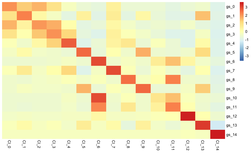
scID provides functions to visualise the results. The next function creates a heatmap of the average expression of each cluster-specific geneset in each of the reference or target clusters clusters. Each row represents a luster-specific geneset and each column a cluster of cells.
So, the following plot shows the expression of cluster-specific genes in the reference dataset
make_heatmap(gem = reference_gem, labels = reference_clusters, markers = scID_output$markers)
and the respective heatmap of target nuclei data grouped by scID is shown below
make_heatmap(gem = target_gem, labels = scID_output$labels, markers = scID_output$markers)
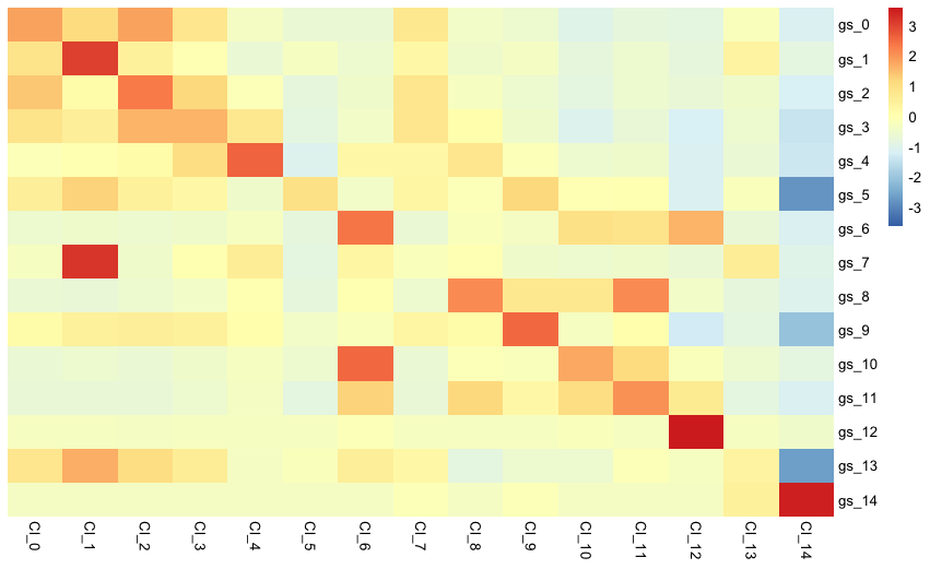
Here we can see that the gene expression pattern in the target data is very similar to the one in the reference data. The gray column shows that no target cell was assigned to the reference clusters 5 and 13.
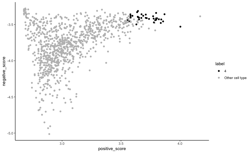
Additionally, for a given reference cluster, selected target cells can be projected onto two dimensions: i) the score for positive markers of the reference cluster and ii) the score for negative markers of the reference clysrer. Matching target cells are expected to be on the top right corner of the plot. Cells are coloured based on the result of scid_multiclass.
For example, the plot for reference cluster 1 from the above result can be obtained as follows:
plot_score_2D(gem = target_gem, labels = scID_output$labels, markers = scID_output$markers,
              clusterID = "4", weights = scID_output$estimated_weights)